Agenda: 1. Normal Distribution 2. It’s Importance 3. Parameters — Mean & Standard Deviation 4. Properties 5. Standard Scores 6. Applications
What is Normal Distribution?
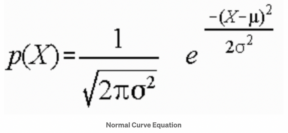
The normal distribution aka Gaussian distribution, is a continuous probability distribution that is described by Normal Equation given below:
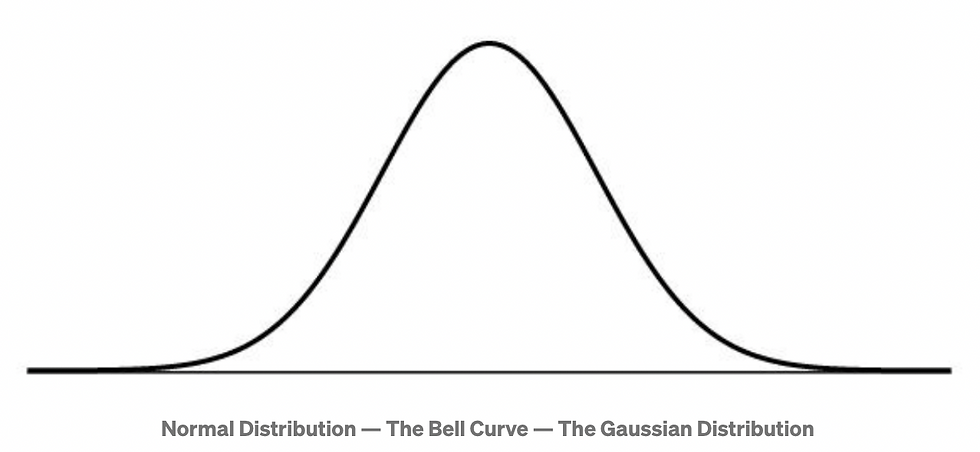
A Normal distribution curve is symmetrical on both sides of the mean, so the right side of the center is a mirror image of the left side.
The area under the normal distribution curve represents probability, and the total area under the curve sums to one.
Normal Distribution — Why is it considered important?
1. The statistical hypothesis test assumes that the data follows a normal distribution. 2. Both linear and non-linear regression assumes that the residual follows the normal distribution. 3. Moreover, the central limit theorem states that as the sample size increases the distribution of the mean follows normal distribution irrespective of the distribution of the original variable
Parameters of Normal Distribution
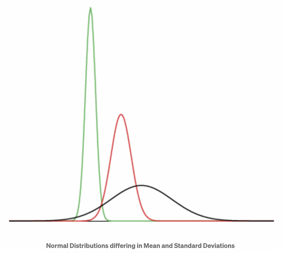
Normal distributions are defined by two parameters, the mean (μ) and the standard deviation (σ).
Mean
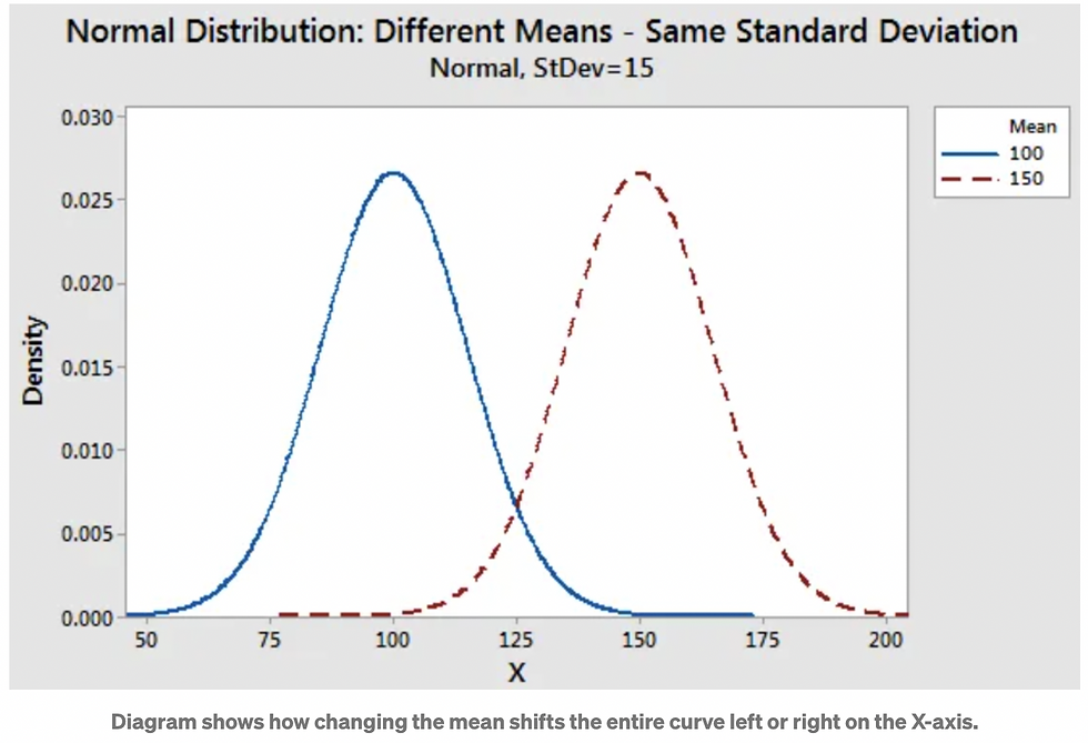
It determines the location of the peak, and most of the data points are clustered around the mean in a normal distribution graph.
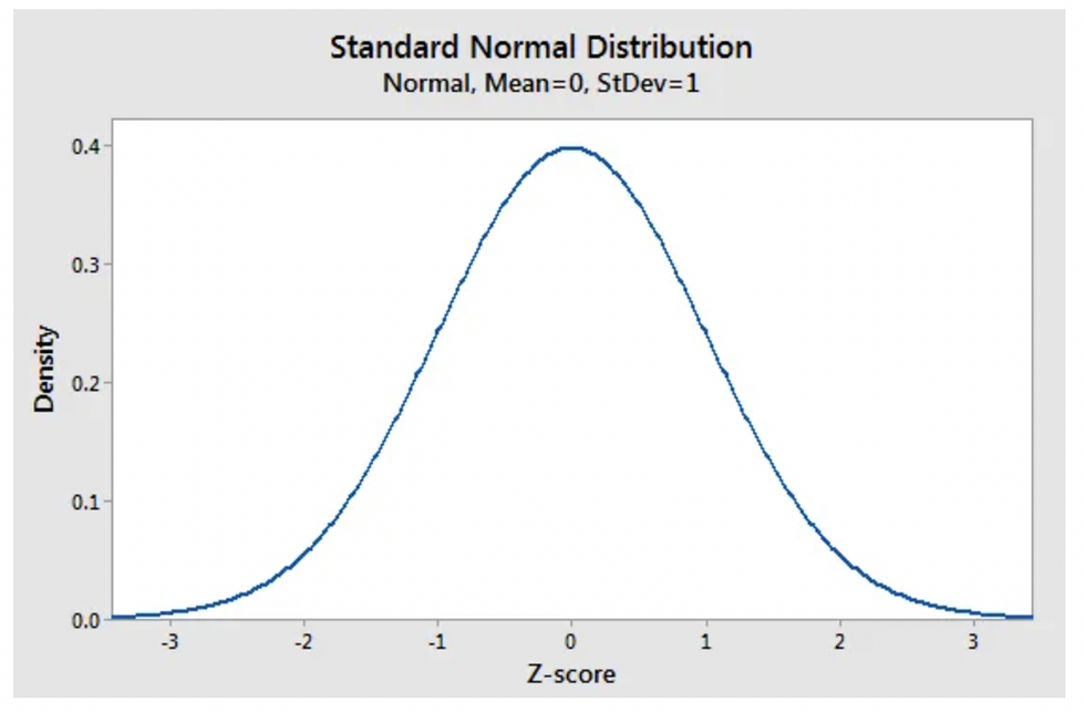
In a standard normal distribution the mean is zero.
On a graph, changing the mean shifts the entire curve left or right on the X-axis.
Standard Deviation
It determines how far the data points are away from the mean and represents the distance between the mean and the data points.
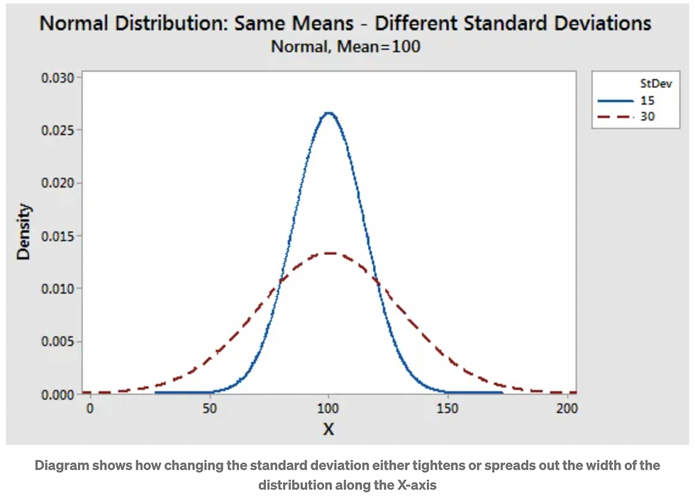
On a graph, changing the standard deviation either tightens or spreads out the width of the distribution along the X-axis. Larger standard deviations produce wider distributions.
In a Standard Normal Distribution, the SD is 1
Properties of Normal Distribution
Mean, Median, and Mode are equal.
The curve is symmetric, with half of the values on the left and half of the values on the right.
The area under the curve is 1.
It has Zero Skewness and Kurtosis is equal to 3 (Mesokurtic)
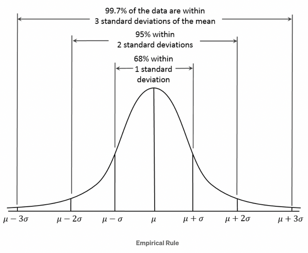
A Normal distribution follows the Empirical rule, which states that:
68% of the data falls within 1 standard deviation of the mean
95% of the data falls within 2 standard deviations of the mean
99.7% of the data falls within 3 standard deviations of the mean.
Standard Scores
A value on the standard normal distribution is known as a Standard Score or a Z-score.
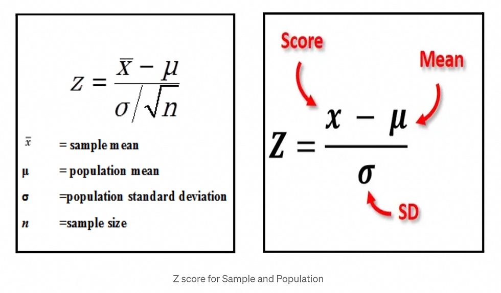
It represents the number of standard deviations above or below the mean that a specific observation falls.
For example, a standard score of 1.5 indicates that the observation is 1.5 standard deviations above the mean. On the other hand, a negative score represents a value below the average. The mean has a Z-score of 0.
Applications
Problem Statement: Let’s have data of heights of Indian men aged 18 to 24, which is approximately normally distributed with a mean of 65.5 inches and a standard deviation of 2.5 inches.
From the empirical rule, it follows that:
– 68% of these Indian men have heights between 65.5–2.5 and 65.5 + 2.5 inches or between 63 and 68 inches,
– 95% of these Indian men have heights between 65.5–2(2.5) and 65.5 + 2(2.5) inches, or between 60.5 and 70.5 inches.
– Therefore, the tallest 2.5% of these men are taller than 70.5 inches. (The extreme 5% fall more than two standard deviations, or 5 inches from the mean. And since all normal distributions are symmetric about their mean, half of these men are on the tall side.)
– Almost all young Indian men are between 58 and 73 inches in height if you use the 99.7% calculations
Thanks for reading 😊

Kommentare